
Recommenders, generally associated with e-commerce, sift though a huge inventory
of available items to find and recommend ones that a user will like. Different
from search, recommenders rely on historical data to tease out user
preference. How does a recommender accomplish this? In this post we explore
building simple recommendation systems in PyTorch using
the Movielens 100K data, which
has 100,000 ratings (1-5) that 943 users provided on 1682 movies.
Matrix Factorization

We first build a traditional recommendation system based on matrix
factorization. The
input data is an interaction matrix where each row represents a user and each
column represents an item. The rating assigned by a user for a particular item
is found in the corresponding row and column of the interaction matrix. This
matrix is generally large but sparse; there are many items and users but a
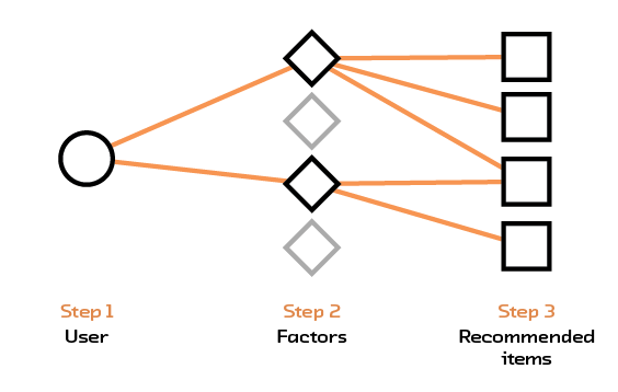
single user would only have interacted with a small subset of items. Matrix
factorization decomposes this larger matrix into two smaller matrices – the
first one maps users into a set of factors and the second maps items into the
same set of factors. Multiplying these two smaller matrices together gives an
approximation to the original matrix, with values for empty elements
inferred. To predict a rating for a user-item pair, we simply multiply the row
representing the user from the first matrix with the column representing the
item from the second matrix.
In PyTorch we can implement a version of matrix factorization by using the
embedding layer to “map” users into a set of factors. The number of factors
determine the size of the embedding vector. Similarly we map items into their
own embedding layer. Both user and item embeddings have the same size. To
predict a user-item rating, we multiply the user embeddings with item embeddings
and sum to obtain one number. The following code draws from Ethan Rosenthal’s
work on matrix factorization in
PyTorch.
import torch
from torch.autograd import Variable

class MatrixFactorization(torch.nn.Module):
    def __init__(self, n_users, n_items, n_factors=20):
        super().__init__()
	# create user embeddings
        self.user_factors = torch.nn.Embedding(n_users, n_factors,
                                               sparse=True)
	# create item embeddings
        self.item_factors = torch.nn.Embedding(n_items, n_factors,
                                               sparse=True)

    def forward(self, user, item):
    	# matrix multiplication
        return (self.user_factors(user)*self.item_factors(item)).sum(1)

    def predict(self, user, item):
        return self.forward(user, item)
To fit the matrix factorization model we need to pick a loss function and an
optimizer. In this example we use the average squared distance between the
prediction and the actual value as a loss function, this is known as
mean-squared error. We then try to minimize this loss by using stochastic
gradient descent. The code below shows how the model is fitted in four steps: i)
pass in a user-item pair, ii) forward pass to compute the predicted rating, iii)
compute the loss, and iv) backpropagate to compute gradients and update the
weights.
model = MatrixFactorization(n_users, n_items, n_factors=20)
loss_fn = torch.nn.MSELoss()
optimizer = torch.optim.SGD(model.parameters(),
                            lr=1e-6)

for user, item in zip(users, items):
    # get user, item and rating data
    rating = Variable(torch.FloatTensor([ratings[user, item]]))
    user = Variable(torch.LongTensor([int(user)]))
    item = Variable(torch.LongTensor([int(item)]))

    # predict
    prediction = model(user, item)
    loss = loss_fn(prediction, rating)

    # backpropagate
    loss.backward()

    # update weights
    optimizer.step()
We train this model on the Movielens dataset with ratings scaled between [0, 1]
to help with convergence. Applied on the test set, we obtain a root mean-squared
error(RMSE) of 0.66. This means that on average, the difference between our
prediction and the actual value is 0.66!
Dense Feedforward Neural Network
Given the underwhelming performance of our matrix factorization model, we try a
simple feedforward recommendation system instead. The input to this neural
network is a pair of user and item represented by their IDs. Both user and item
IDs first pass through an embedding layer. The output of the embedding layer,
which are two embedding vectors, are then concatenated into one and passed into
a linear network. The output of the linear network is one dimensional –
representing the rating for the user-item pair. The model is fit the same way as
the matrix factorization model and uses the standard PyTorch approach of forward
passing, computing the loss, backpropagating and updating weights.
import torch
import torch.nn.functional as F
from torch.autograd import Variable
from torch import nn

class DenseNet(nn.Module):

    def __init__(self, n_users, n_items, n_factors, H1, D_out):
        """
        Simple Feedforward with Embeddings
        """
        super().__init__()
   	# user and item embedding layers
        self.user_factors = torch.nn.Embedding(n_users, n_factors,
                                               sparse=True)
        self.item_factors = torch.nn.Embedding(n_items, n_factors,
                                               sparse=True)
   	# linear layers
        self.linear1 = torch.nn.Linear(n_factors*2, H1)
        self.linear2 = torch.nn.Linear(H1, D_out)

    def forward(self, users, items):
        users_embedding = self.user_factors(users)
        items_embedding = self.item_factors(items)
	# concatenate user and item embeddings to form input
        x = torch.cat([users_embedding, items_embedding], 1)
        h1_relu = F.relu(self.linear1(x))
        output_scores = self.linear2(h1_relu)
        return output_scores

    def predict(self, users, items):
        # return the score
        output_scores = self.forward(users, items)
        return output_scores
Once again, we train this model on the Movielens dataset with ratings scaled
between [0, 1] to help with convergence. Applied on the test set, we obtain a
root mean-squared error(RMSE) of 0.28, a substantial improvement!
Sequence based Recommendation System
Finally we build a recommendation system that takes into account the sequence of
item interactions. The heart of this is a Long Short-Term Memory (LSTM) cell, a
variant of Recurrent Neural Networks (RNN) with faster convergence and better
long term memory. The input to this system is a history of item interactions and
their corresponding ratings. In the following example of an input, we show a
sequence of item interaction of length 10 (arbitrarily chosen) and the
corresponding rating. Elements in the first array correspond to items(movies),
and elements in the second array correspond to ratings. We see that, for
example, movie 209 has a rating of 4, and movie 32 has a rating of 5. Sequences
shorter than 10 are padded with zeros.
In [2]: training_data[0]
Out[2]:
(array([209,  32, 189, 242, 171, 111, 256,   5,  74, 102], dtype=int32),
 array([4, 5, 3, 5, 5, 5, 4, 3, 1, 2], dtype=int32))
Items are passed through an embedding layer before going into the LSTM. The
output of the LSTM is then fed into a linear layer with an output dimension of
one. The LSTM has 2 hidden states, one for short term memory and one for long
term. Both states need to be initialized.
PyTorch expects LSTM inputs to be a three dimensional tensor. The first
dimension is the length of the sequence itself, the second represents the number
of instances in a mini-batch, the third is the size of the actual input into the
LSTM. Using our training data example with sequence of length 10 and embedding
dimension of 20, input to the LSTM is a tensor of size 10x1x20 when we do not
use mini batches. For a mini-batch size of 2, each forward pass will have two
sequences, and the input to the LSTM needs to have a dimension of 10x2x20. LSTMs
take variable input sequence lengths but for batch training purposes the input
data is generally processed(with padding if necessary) to have a fixed length.
import torch
import torch.nn as nn
from torch.autograd import Variable

class LSTMRating(nn.Module):

    def __init__(self, embedding_dim, hidden_dim, num_items, num_output):
        super().__init__()
        self.hidden_dim = hidden_dim
        self.item_embeddings = nn.Embedding(num_items, embedding_dim)
        self.lstm = nn.LSTM(embedding_dim, hidden_dim)
        self.linear = nn.Linear(hidden_dim, num_output)
        self.hidden = self.init_hidden()

    def init_hidden(self):
    	# initialize both hidden layers
        return (Variable(torch.zeros(1, 1, self.hidden_dim)),
                Variable(torch.zeros(1, 1, self.hidden_dim)))

    def forward(self, sequence):
        embeddings = self.item_embeddings(sequence)
        output, self.hidden = self.lstm(embeddings.view(len(sequence), 1, -1),
                                        self.hidden)
        rating_scores = self.linear(output.view(len(sequence), -1))
        return rating_scores

    def predict(self, sequence):
        rating_scores = self.forward(sequence)
        return rating_scores
Once the neural network is defined, we fit the training data using stochastic
gradient descent with a mean squared error loss function.
embedding_dim = 64
hidden_dim = 128
n_output = 1

# add one to represent padding when there is not enough history
model = LSTMRating(embedding_dim, hidden_dim, n_items+1, n_output)
loss_fn = nn.MSELoss()
optimizer = optim.SGD(model.parameters(), lr=0.1)

for sequence, target_ratings in training_data:
    model.zero_grad()
    # initialize hidden layers
    model.hidden = model.init_hidden()
    # convert sequence to PyTorch variables
    sequence_var = Variable(torch.LongTensor(sequence.astype('int64')))
    # forward pass
    ratings_scores = model(sequence_var)
    target_ratings_var = Variable(torch.FloatTensor(target_ratings.astype('float32')))
    # compute loss
    loss = loss_fn(ratings_scores, target_ratings_var)
    # backpropagate
    loss.backward()
    # update weights
    optimizer.step()
Similar to other models, we train the LSTM-based model on the Movielens dataset
with ratings scaled between [0, 1] to help with convergence. Applied on the test
set, we obtain a root mean-squared error(RMSE) of 0.43 – the LSTM model
underperforms the dense feed forward network.
Post-amble
The models discussed in this post are basic building blocks for a recommendation
system in PyTorch. There are no bells and whistles and we did not attempt to
fine tune any hyperparameters. Our first pass result suggests that the dense
network performs best, followed by the LSTM network and finally the matrix
factorization model. The root mean-squared error (RMSE) are 0.28, 0.43 and 0.66
respectively on the Movielens 100K dataset with ratings scaled between [0,
1]. We thought PyTorch was fun to use; models can be built and swapped out
relatively easily. When we did encounter errors, most of them were triggered by
incorrect data types.
For more on recommendations, please see our Semantic Recommendations report
where we focus on how machines can better understand content!